


This insight builds upon the theoretical basis given in our previous INSIGHT “FROM ANTENNA TO GNSS RECEIVER” but focuses on real world measurements and how to perform them with off-the-shelf GNSS receivers. So this document is more a practical application of the theory explained. If you have not yet read the previous INSIGHT please do so first. This document enables you to do actual measurements on your setup with equipment that you might already own. There is no need to purchase expensive equipment to verify or debug your setup from a perspective of signal levels. So practical issues as verifying whether your GNSS amplifier is giving you the gain you require or verifying the cable loss you calculated matches the installed cable will be addressed in this document.
We have prepared several scenarios with different signal levels and signal to noise ratios. Each of the four scenarios adds something to the setup that is used to explain certain aspects.
| Scenario | |
|---|---|
| A | GNSS receiver with nothing connected |
| B | GNSS receiver connected to antenna and a long cable |
| C | GNSS receiver connected to a long cable with an amplifier just before the receiver (scenario B + amplifier) |
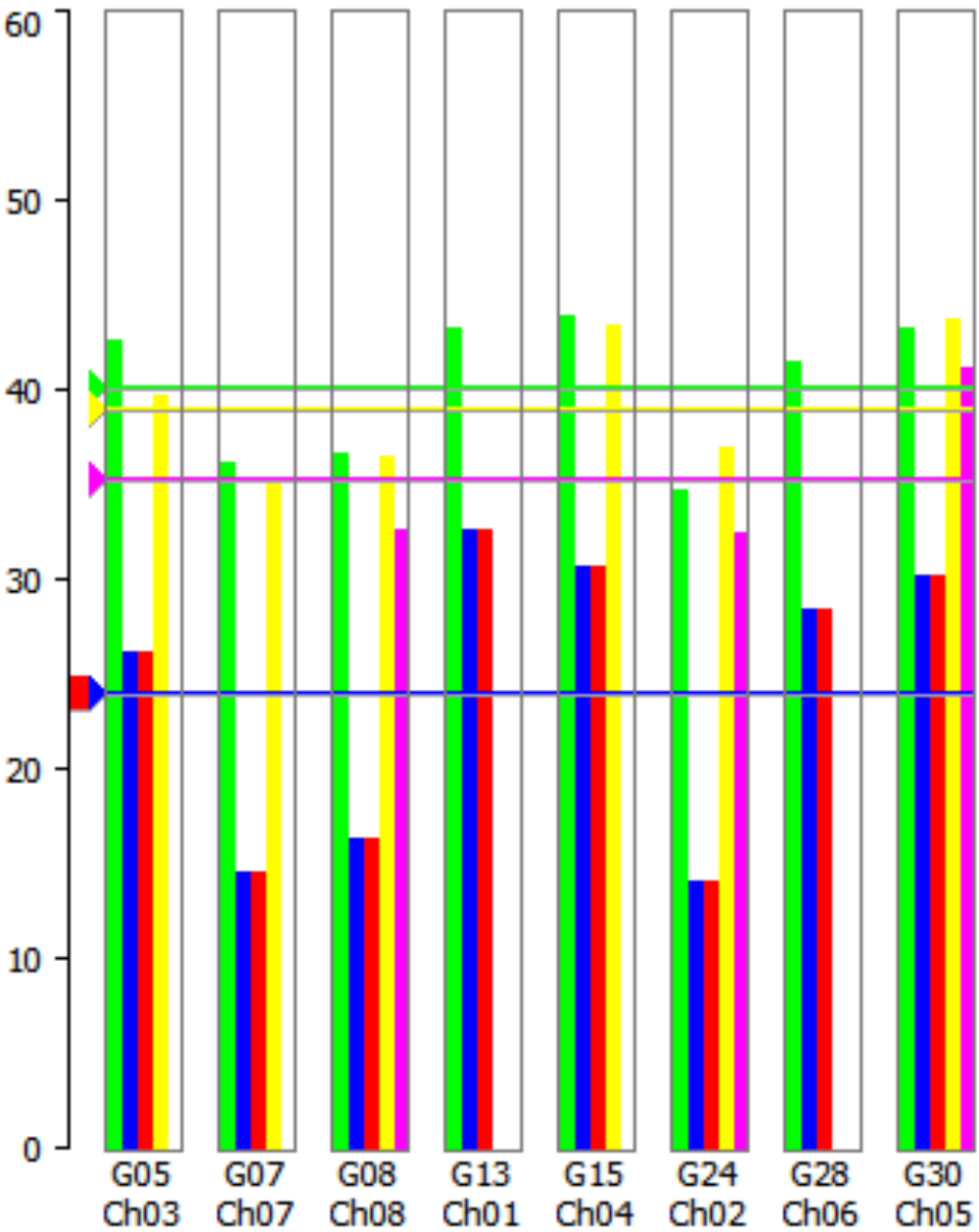
| D | GNSS receiver connected to a long cable with two amplifiers just before the receiver (scenario C + amplifier) |
The methods here explained can be applied on our GNSS receivers with Septentrio boards inside. The screen captures are taken from RxControl, an application designed by Septentrio to allow an easy and productive interaction with Septentrio receivers. The principle can of course be applied to every GNSS receiver that has an AGC amplifier that can be monitored.

To get an understanding on how the built-in AGC amplifier works, the simplest setup is just looking at a receiver that has no input signals. As explained in the previous INSIGHT, the AGC amplifier will try to provide a constant output power to the rest of the GNSS receiver. Because there is no input signal present, the AGC amplifier will regulate itself to maximum gain. So looking at these levels, they indicate the maximum GAIN you can obtain with your receiver. These are an interesting baseline to compare other measurements with. We suggest always performing this measurement first.
")
The screen capture above shows the AGC Gain levels for every front end that is available in the GNSS receiver. This specific receiver shows 6 individual AGC levels. In this INSIGHT we will always look at the GPSL1/E1 signal. The same logic can be applied to the other front ends but just looking at one is enough for this use case. So we now know that the maximum gain level of this receiver on GPSL1/E1 is 59dB.

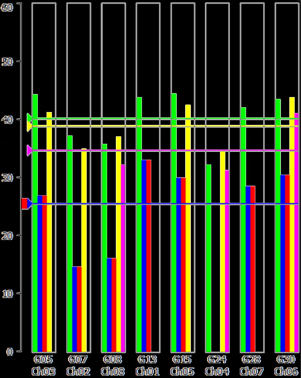
This scenario was built to demonstrate the effect of a very low signal level on the input of a GNSS receiver. We got to this point by adding cable length to the point that the AGC amplifiers were almost maxed out. So at this point the amplifier in the GNSS receiver could go not much further. As you can see on the capture below, the amplifier for GPSL1/E1 is only 2dB under his maximum gain.

As you can imagine, having the AGC amps maxed out means that you are operating on the limits of the receiver. When using a receiver with a Septentrio board inside, you can always have a quick look at the quality view.
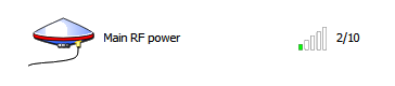
As you can see, it indicated that the RF power at the main antenna is at 2/10. Although this is just a rough quality indicator, this can be very helpfull to make a quick analysis of your setup. Of course the target should be to get a 10/10 on RF power on the input of the GNSS receiver.
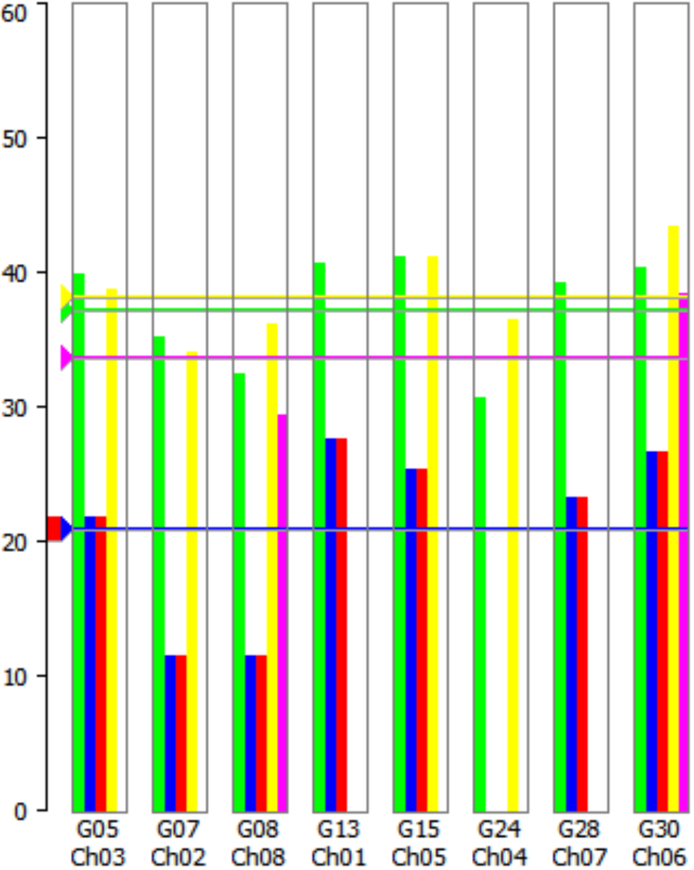
In this scenario there are GNSS signals received by the receiver and thus Signal to Noise values are determined by the receiver. What we would like to demonstrate with this scenario is that although the AGC still has a few extra dB available and thus is not maxed out we see lower values then we would expect. You can compare them with the scenarios to come and you will see that they are higher. This has to do with the noise figure of the receiver. As explained in our previous INSIGHT, a GNSS receiver has a higher noise figure than an amplifier. So please note that if we would insert an amplifier before the GNSS receiver, we would get better signal to noise values as we will demonstrate below. This is because the noise figure of the amplifier is lower than the noise figure of the GNSS receiver.
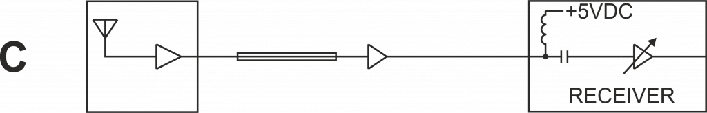
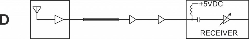
This scenario is created from scenario B by just adding an amplifier just before the GNSS receiver. Adding this amplifier improves the signal to noise ratio determined by the GNSS receiver and as you would expect changes the AGC values of the receiver. Lets first have a look at the AGC table:

The amplifier we added is a 20dB amplifier. Since this amplifier comes in series with the AGC amplifier, the sum of both amplifier gains must be the same in these scenarios. Since we now have added 20dB, the AGC will regulate 20dB down to get the same output level. The gain on GPSL1/E1 has changed from 57dB to 37dB. So the AGC is doing his job perfectly by compensating the input signal to a constant output signal. In this scenario we know the gain of the amplifier, but these AGC tables can of course be used in the opposite direction. If you have for example in your setup a cable that has an attenuation (cable loss) that you would like to verify. You can measure the AGC values before and after the cable and the compare them. The extra gain that the AGC introduces in this case represents the cable loss introduced by the cable. Please note that for this to be true, you need to keep away from the low and high limits of the AGC!
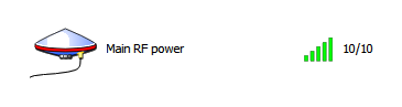
If you now take a look at the quality view you will find that the RF power at the main antenna should be 10/10. The 20dB amplification that has been added brings the signal up high enough to be in the intended range of input levels of the receiver.
In this scenario you can see that the signal to noise values determined by the GNSS receiver are significant better compared to scenario B. This is because the noise figure of the amplifier is lower than the noise figure of the GNSS receiver. Please note that the actual signal to noise levels in scenario B were better then what the GNSS receiver could make of them. So it is the wrong to think that the amplifier improved the signal to noise ratio of the signal! It is however correct to think that the amplifier has a lower noise figure and therefore is able to amplify the signal to a level where the GNSS receiver is capable of working with it without significant signal to noise deterioration.
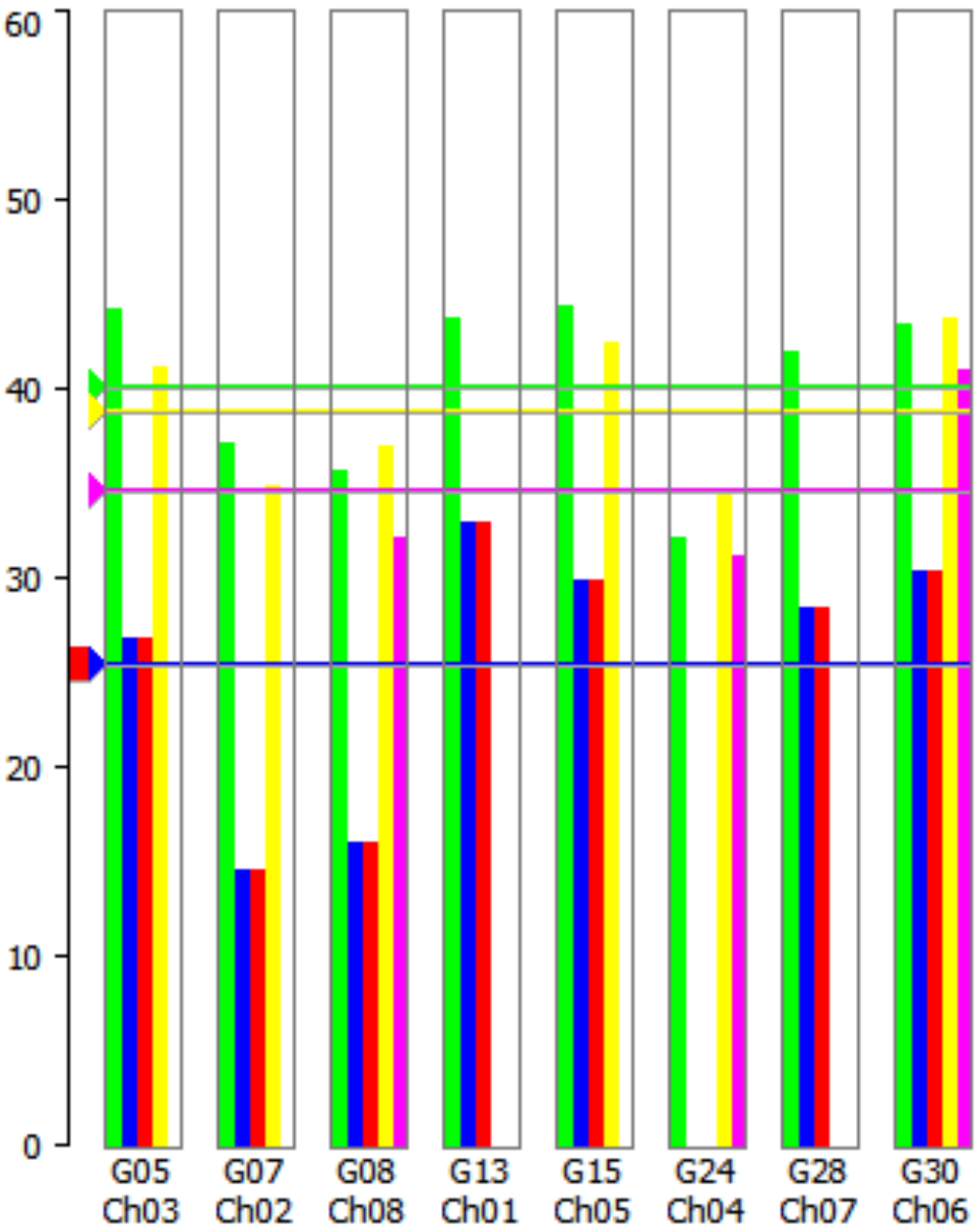
In this last scenario we have added another amplifier to the signal chain. We have created this scenario to demonstrate two things. First the aspect of the AGC levels that as you would expect drop another 20dB. Second you can see that adding the second amplifier has no visual effect on the signal to noise ratio. This is of course a scenario that is purely created to explain some effects and is not recommended.
Lets first have a look at the AGC table:

The amplifier we added is again a 20dB amplifier. So now there are two 20 dB amplifiers installed after each other. The AGC amplifier again regulates itself back 20dB to compensate for the extra added gain in the signal chain. It is not exactly 20dB as you will notice but rather 21dB. The gain of the amplifier is of course not perfectly 20dB and also these are just readings from AGC amplifiers that are not laboratory grade equipment but still give a very usable indication.
In this scenario you can see that there is no significant chance in the signal to noise level compared to scenario C. As we explained in the previous INSIGHT “FROM ANTENNA TO GNSS RECEIVER”, noise at the input is also amplified by the amplifier together with the signal at the input. Every amplifier also adds some noise to the total. When the noise levels at the input are high enough, there is no noticeable chance in the signal to noise ratio after the amplifier compared to the input. This is of course also true for the GNSS receiver. The noise figure of the GNSS receiver does not matter that much after the signal has been amplified.
The method used in scenario C and D to determine the GAIN of the amplifier can of course be used for other purposes. If you have for example in your setup a cable that has an attenuation (cable loss) that you would like to verify. You can measure the AGC values before and after the cable and then compare them. The extra gain that the AGC introduces represents the cable loss introduced by the cable. Please note that for this to be true, you need to keep away from the low and high limits of the AGC!
This INSIGHT discribes and verifies a method that can be used to determine the gain of a GNSS amplifier, the loss of a cable or any other part that you might encounter in your signal path. It enables users of high end GNSS receivers to verify or debug their GNSS signal path. Moreover we have demonstrated basic RF principles as explained in our previous INSIGHT “FROM ANTENNA TO GNSS RECEIVER” in an application with real world measurements.

